In this project, I played around with 2D convolutions and filtering. This included using frequencies in different ways to blur, sharpen, and combine images, as well as implementing Gaussian and Laplacian stacks. Enjoy!
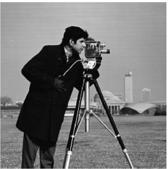
First, let's look at this cameraman image.

We can show the partial derivative in x and y of him by convolving the image with finite difference operators D_x and D_y. On the right, the binarized gradient magnitude image is shown.
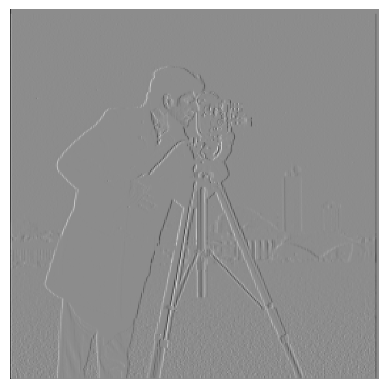
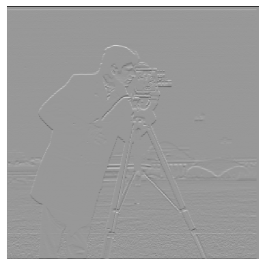
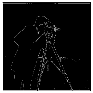
Here, I created a blurred version of the original cameraman image by convolving with a gaussian. The procedure in the previous part was repeated, but now I can see an improved difference in the smoothness and thickness of the edges.
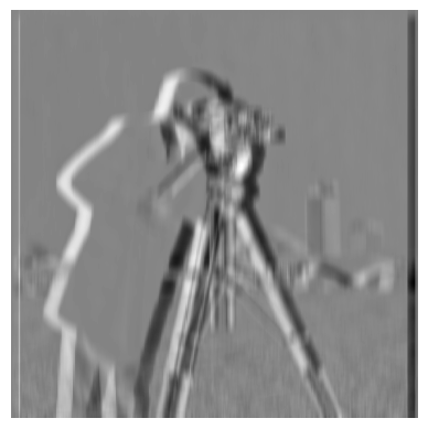
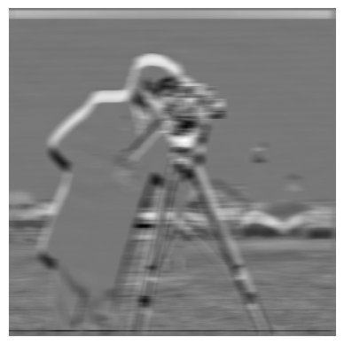
I can do the same thing with a single convolution instead of two, just by creating a derivative of gaussian filters. This gives the exact same result as before! MSE of both images compared to their previous counterparts is <0.005.
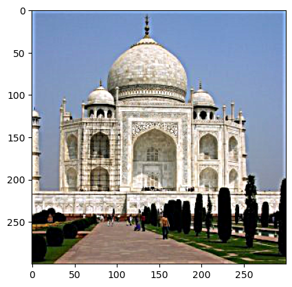
In this part, I derived the unsharp masking technique. We can subtract the blurred version of an image from the original to get the high frequencies of the image. An image often looks sharper if it has stronger high frequencies! See this example with the beautiful Taj Mahal:

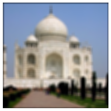
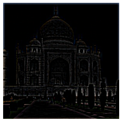
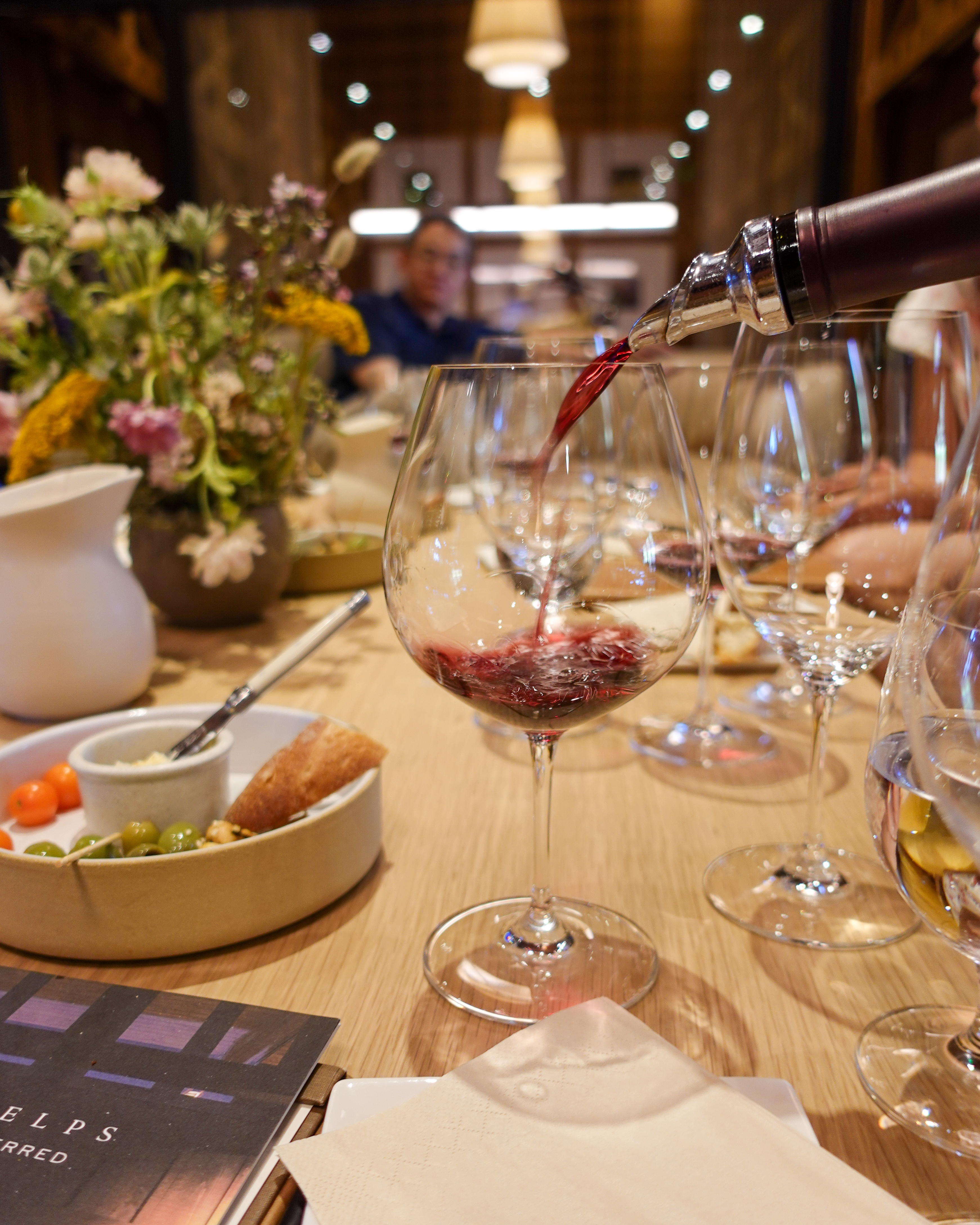
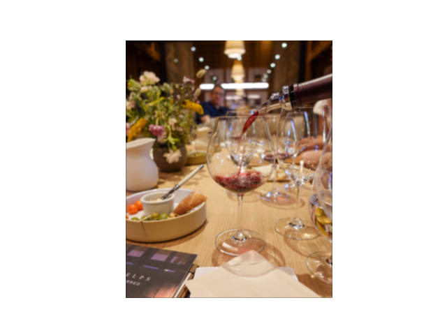
Nice. For evaluation, let's blur and then sharpen this picture I snapped with my camera at Napa Valley:

And another one with my roommate, Coh, who came to Napa with me:
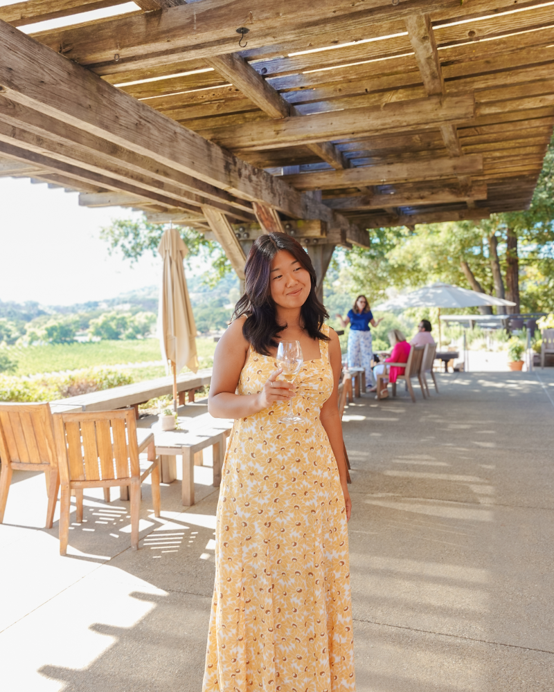
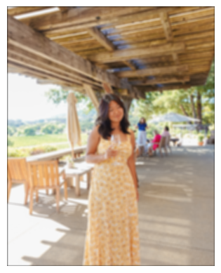
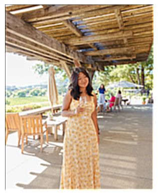
The wine is looking nice and sharp! But Coh could use some adjustment on how much of her high frequencies we're adding.
In this part, I attempted to create hybrid images using the approach described in the SIGGRAPH 2006 paper by Oliva, Torralba, and Schyns. By blending the high frequency portion of one image with the low-frequency portion of another, you can get a hybrid image that leads to different interpretations at different distances!
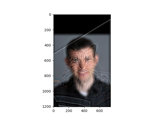
Let's blend Derek and his cat Nutmeg by taking the low frequencies of Derek and the high frequencies of Nutmeg.
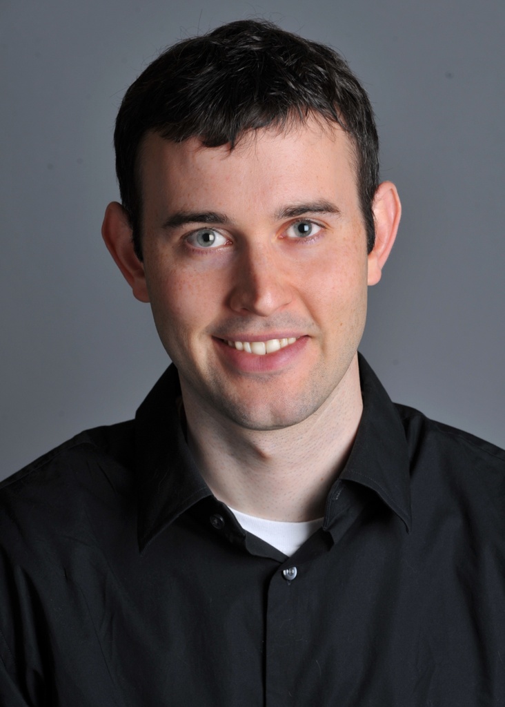
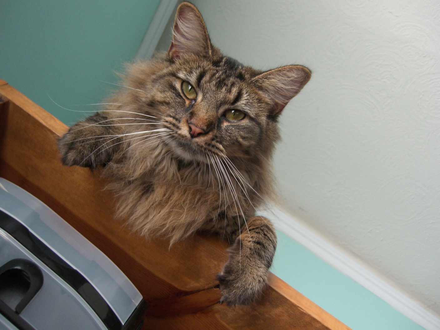
I'm feeling hungry, so let's turn my roommate Coh from earlier into a ear of corn.

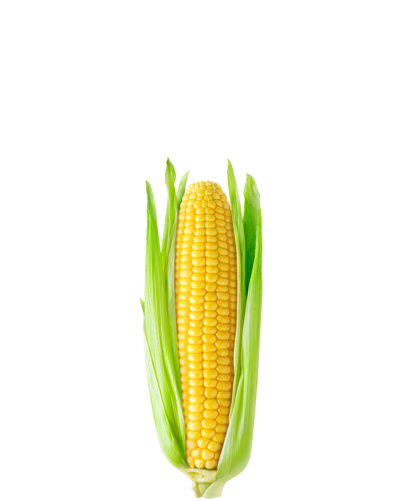
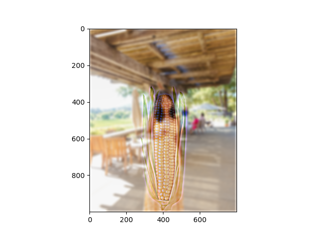
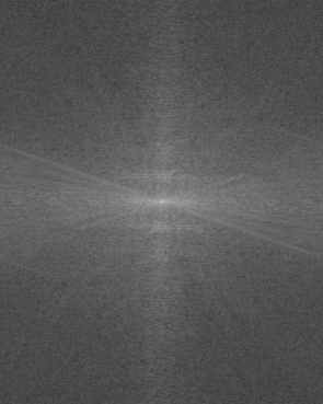
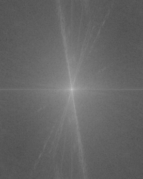
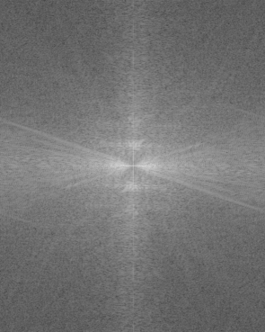
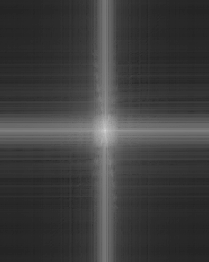
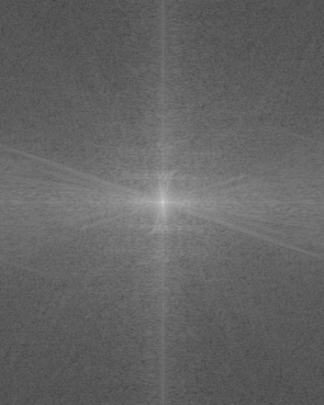
For Cohrn, we can illustrate the process through frequency analysis. Shown here is the log magnitude of the Fourier transform of the two input images, the filtered images, and the hybrid image.


Let's make an Oraple. Here's my Figure 3.4.2

Still hungry, so here's pasta and soup combined.


