In this project, I continued to play with different aspects of image warping. In particular, I learned how to compute homographies to perform image mosaicing. Image mosaics were created by registering, projective warping, resampling, and compositing two or more images that I took.
Before I could warp my images into alignment, I needed to recover the parameters of the transformation between each pair of images. This transformation is a homography: p’ = Hp, where H is a 3x3 matrix with 8 degrees of freedom (the lower right corner is a scaling factor, and can be set to 1). I recovered the homography for my image pairs by (1) manually creating a set of of (p’,p) pairs of corresponding points, and (2) using them as input parameters in the function:
H = computeH(im1_pts, im2_pts)im1_pts and im2_pts are n-by-2 matrices holding the (x, y) locations of n point correspondences from the two images. H is the recovered 3x3 homography matrix.
Now that I have the parameters of the homography, I can use the homography to warp each image towards the reference image. Let's create another function: imwarped = warpImage(im, H), where im is the input image to be warped and H is the homography. I used scipy.interpolate.griddata along with inverse warping in my warpImage function and marked pixels without any mapped values as NaN (black).
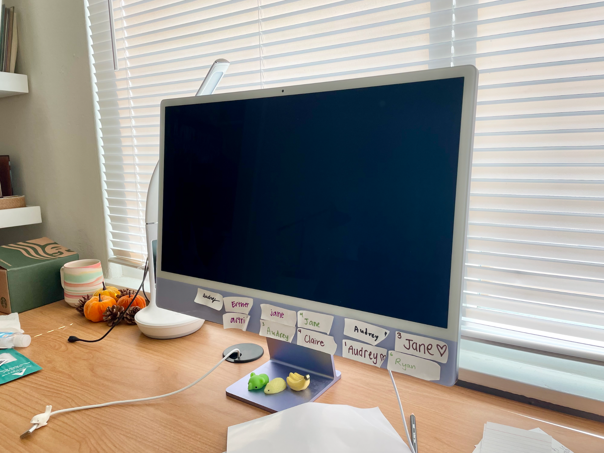
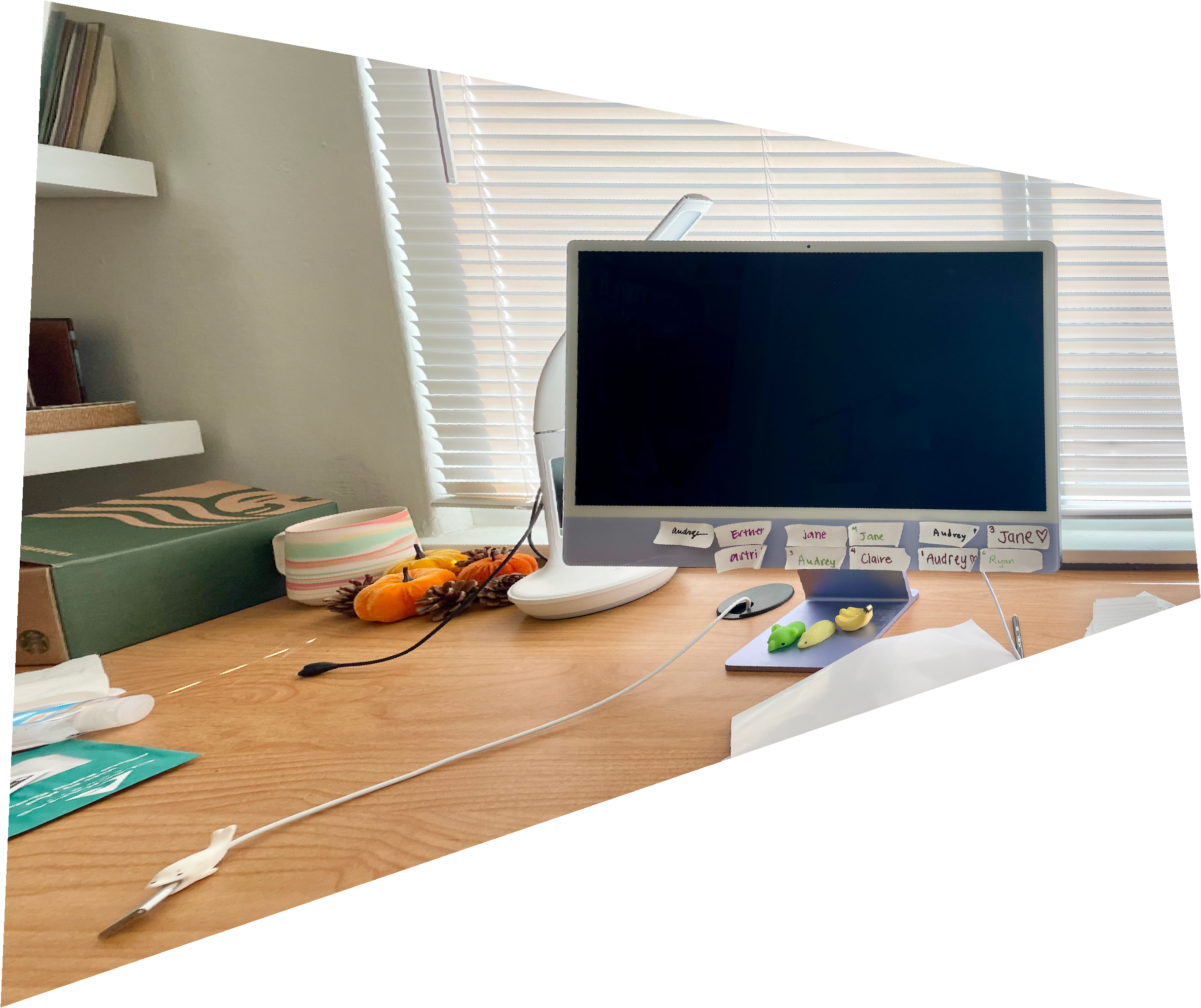
To check if everything was working correctly, I tested my code by performing "rectification" on an image of my monitor.


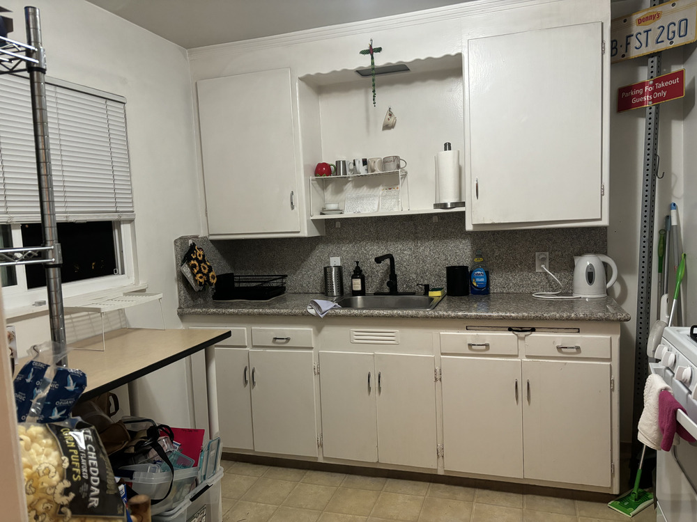
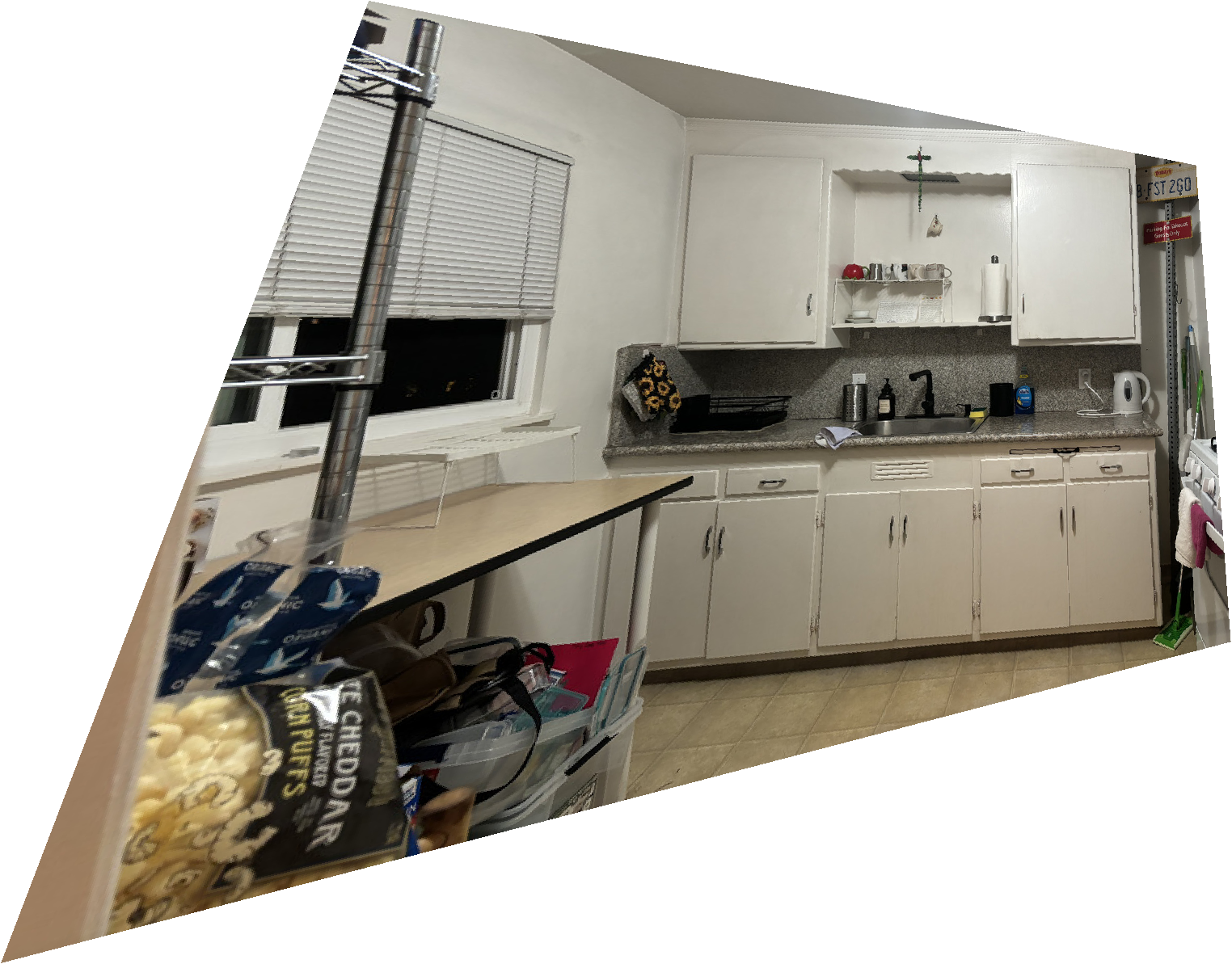
Looks good! I know my monitor is a rectangle in real life, so I just used the four corners of the screen to compute a homography and warp it into an actual rectangle. I can do a similar rectification with this little cupboard area above my kitchen sink:
Let's now create an image mosaic of my living room. I'll start out by taking these two pictures:
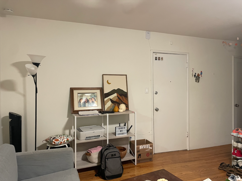
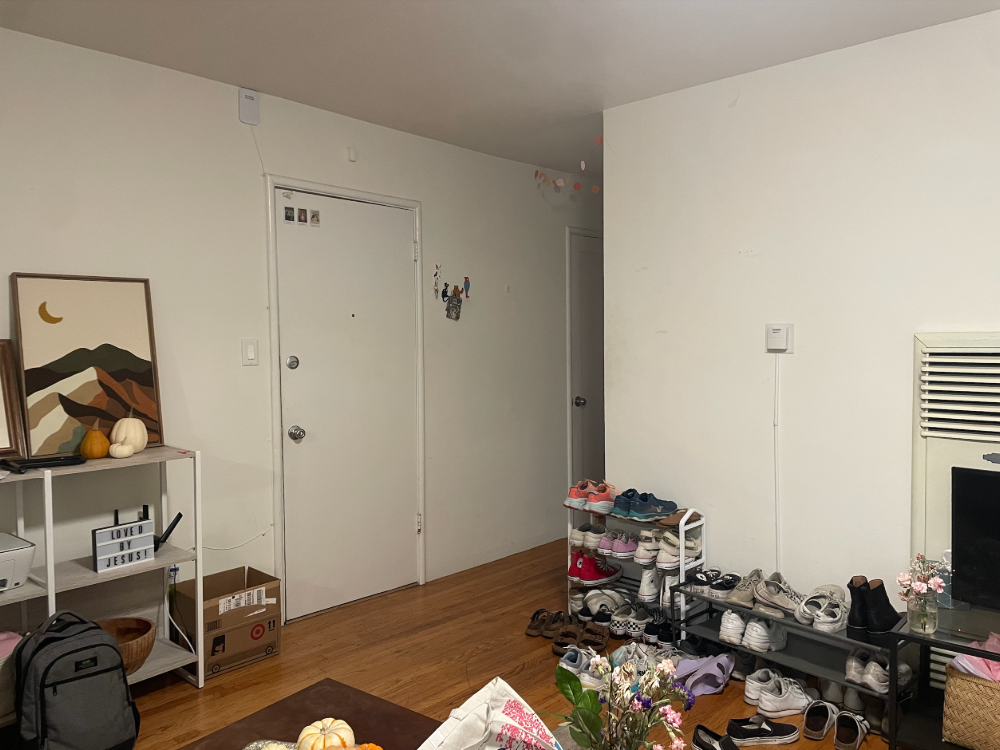
Using the method above, I can warp the first image of my living room to the world of the second image.
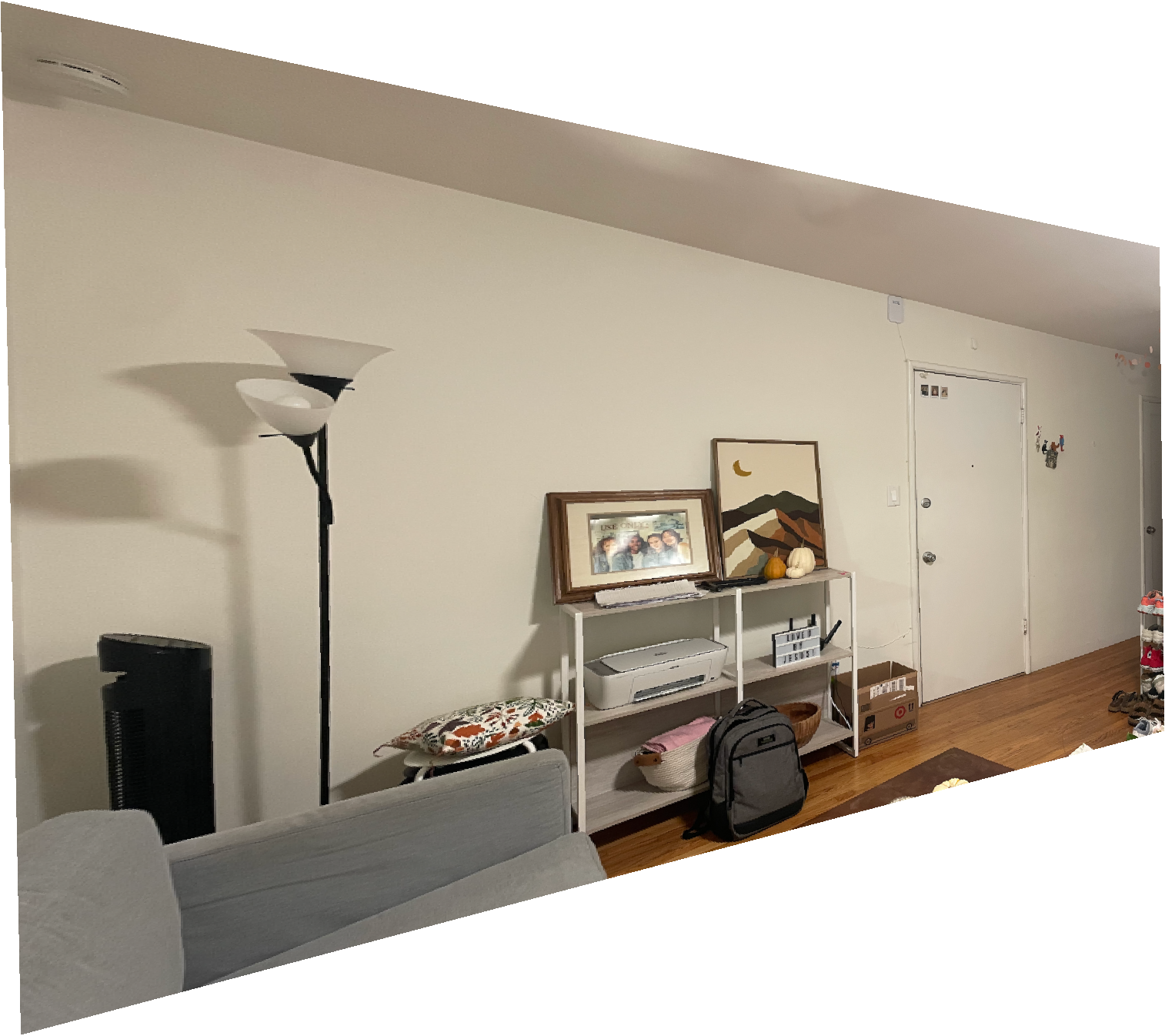
Nice. They can now perfectly overlap.
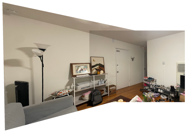
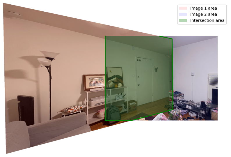
But wait. It's pretty obvious that we're just overlaying two images on top of each other, even though we have warped the first perfectly to the second with the homography. We can try and make this smoother with a simple vertical blending mask, or make use of the scipy.ndimage.distance_transform_edt function (mimicks MATLAB's bwdist function) to create a distance mask, where an alpha value weighs each pixel based on its distance from the centers of the images.

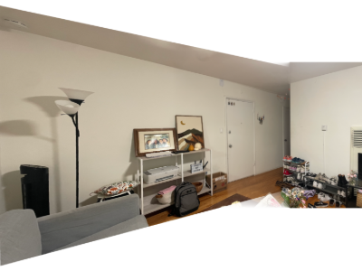
bwdist-like blendingThe second option looks pretty nice, so let's crop it to look more like a smooth paranoma:
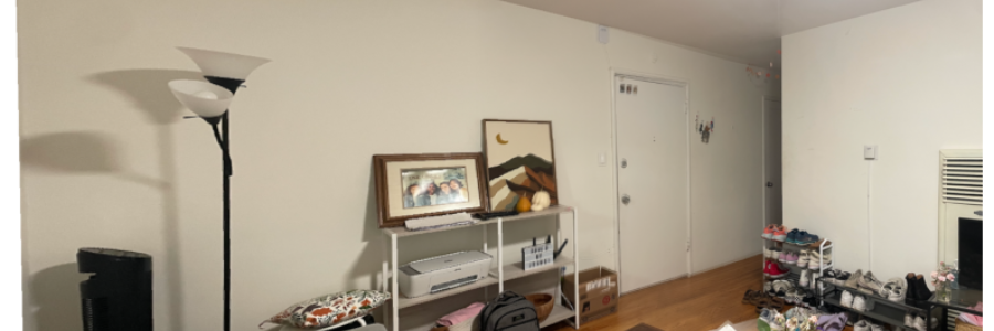
Another with the couch in the living room:
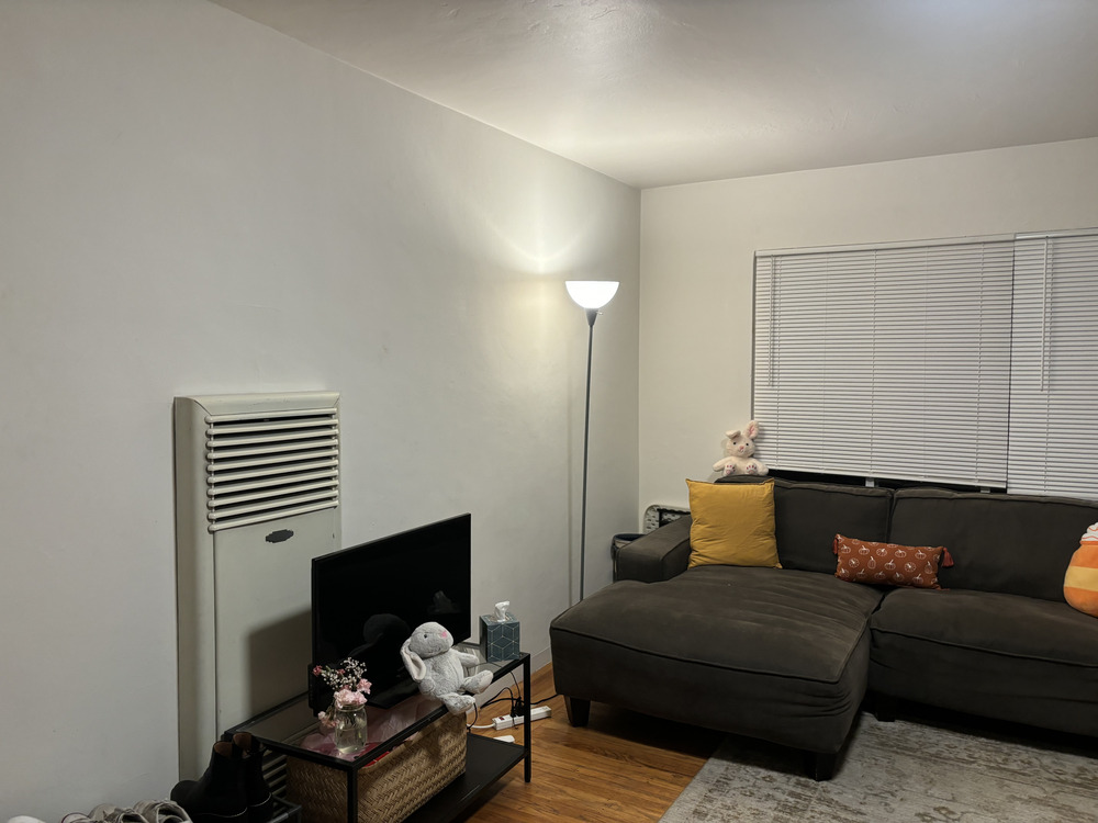
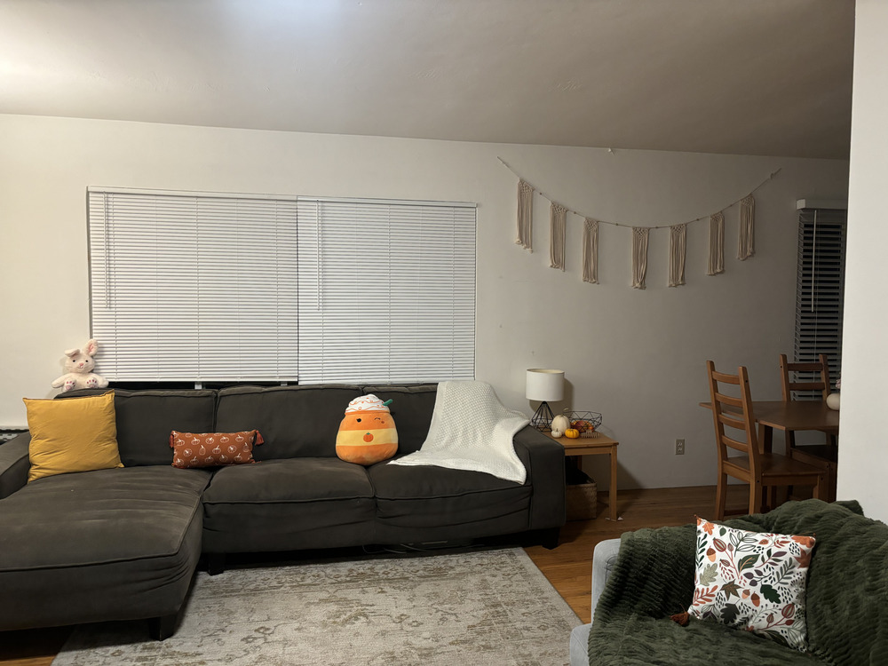
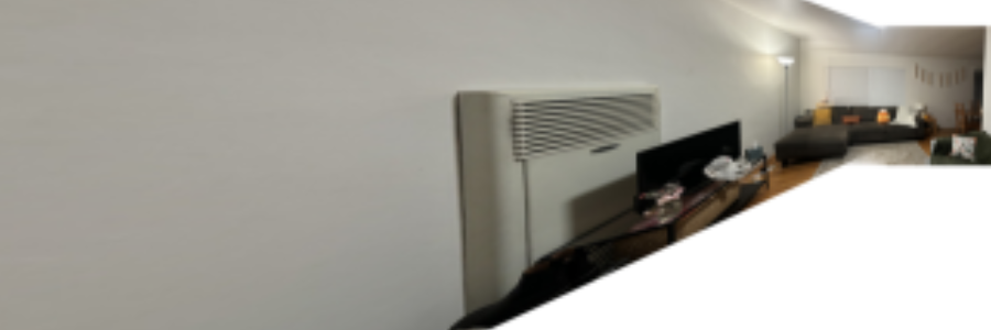
The warped image becomes very large and warped because the rotation from the first image to the second was relatively wide. Here's another one of a chocolate wall I saw in a candy shop in downtown SLO!
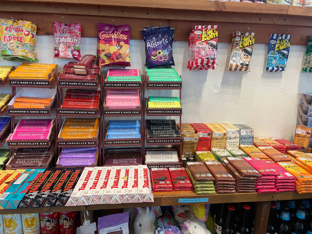
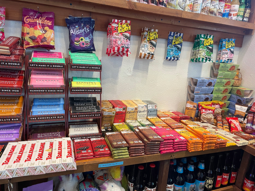
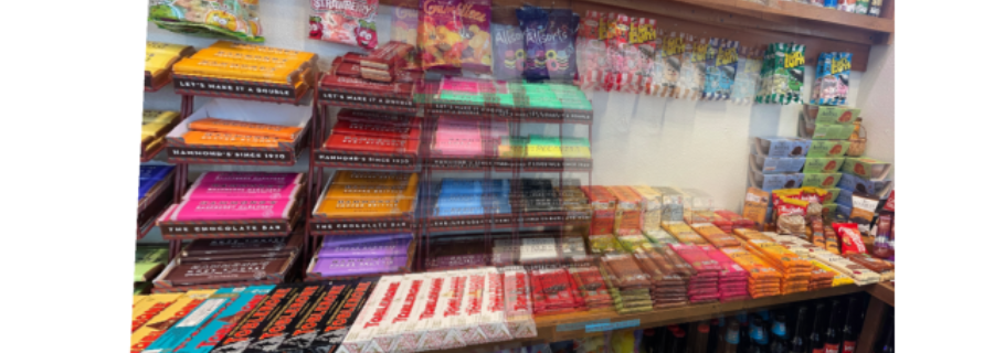
This one turns out a little blurrier because the original photos were pretty complex (it was also hard to rotate perfectly and not shift the center of my phone camera too much).
And another of my apartment's dining area:
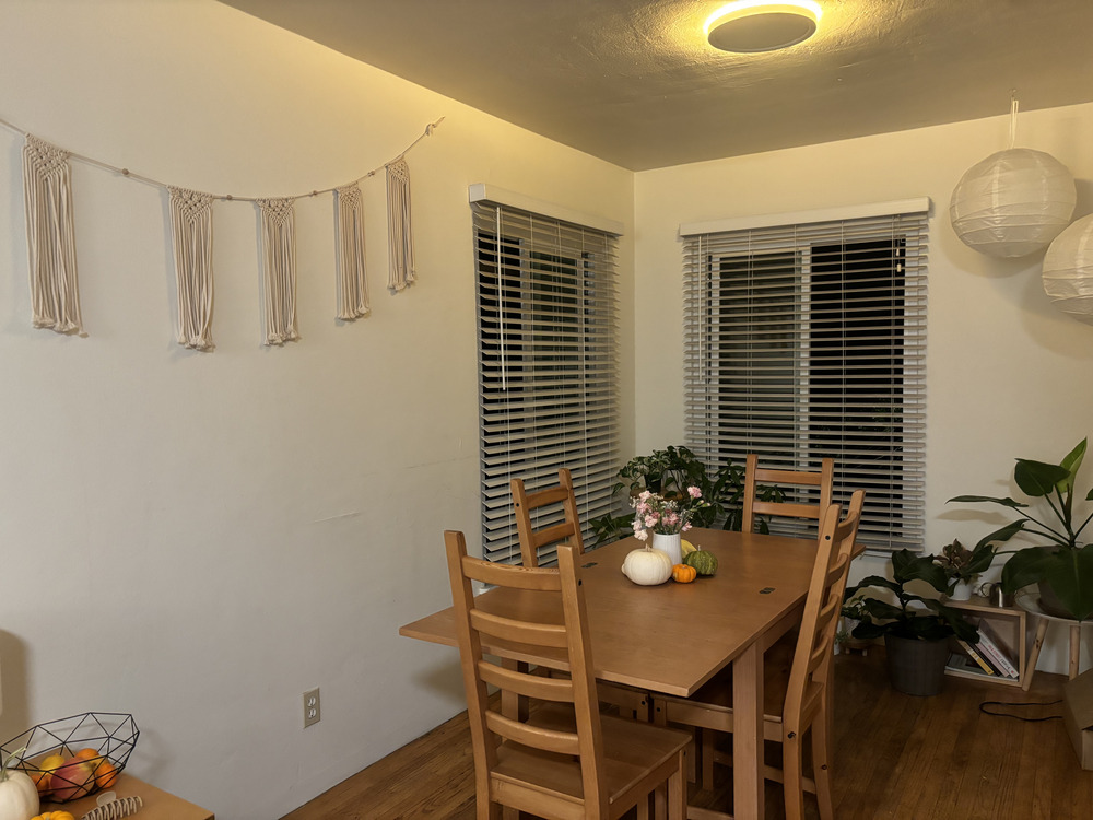
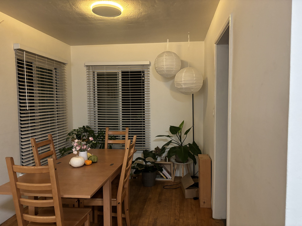
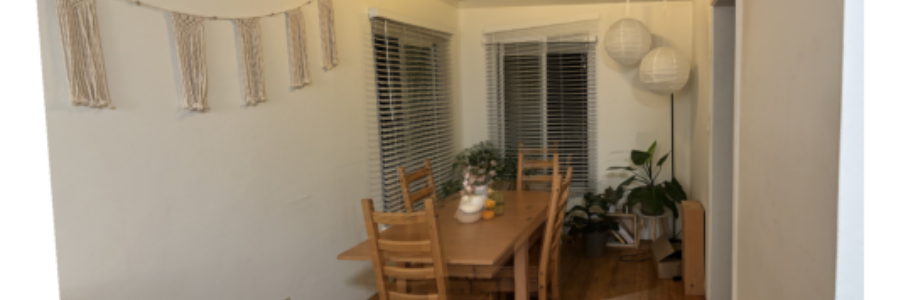
It's a pain to have to manually choose points everytime, so it'd be cool to just automate the point stitching process (and then compute the homography, combine, and blend using the methods above). To automate, we'll follow the process outlined in “Multi-Image Matching using Multi-Scale Oriented Patches” by Brown et al.
First, we will detect Harris corners like how Section 2 (Harris Interest Point Detectors) was mentioned in the paper. Here are Harris corners overlaid on the study room I'm currently working in.
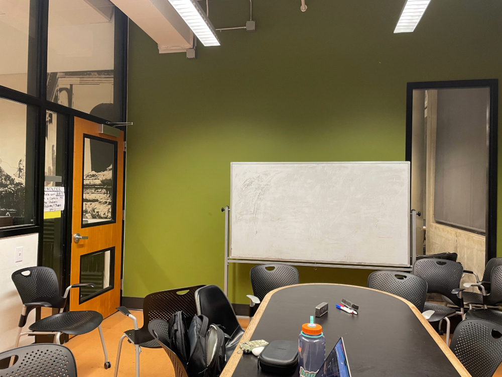
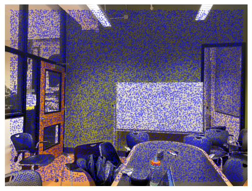
That's a lot of points. Let's implement Adaptive Non-Maximal Suppression (from Section 3 of the Brown paper), so that we can narrow it down to a smaller amount to input into RANSAC after this.
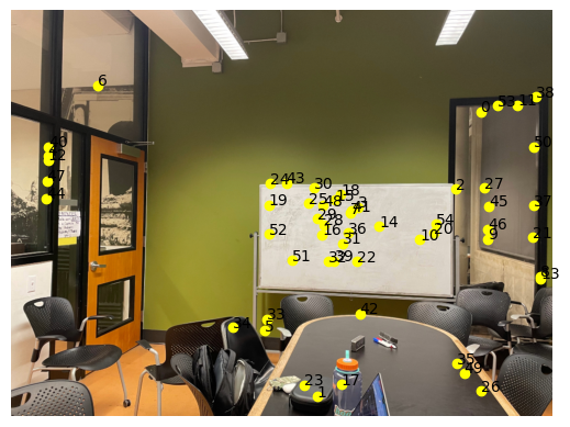
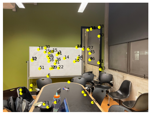
That's still a lot of points! And some of them aren't perfectly aligned. After this we will match feature descriptors by using the surrounding areas around each point (feature patches) as 64-dimensional vectors. We can compute the 1-NN and 2-NN of each feature patch using Euclidean distance as a metric, and use the Lowe ratio to determine a "good match": if the distance of the 1-NN divided by the distance of the 2-NN is less than our ratio (e.g. 0.7), then we know the 1-NN patch in the other image is likely to be a pretty good match given the surrounding context.
To detail my extract_feature_descriptors and match_features functions a little, I implemented Gaussian blurring and anti-aliasing before sampling a 40x40 patch down to 8x8. I chose to do this for each of the 3 RGB channels (then normalizing) rather than just grayscale to get slightly improved matching results.
After this, we'll still have quite a few patches, so that's why we have one more step with RANSAC (random sample consensus) to narrow it down even further.
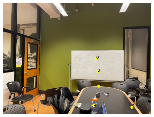
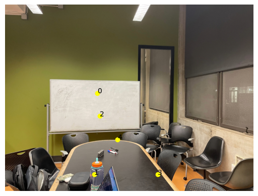
Quick overview of what RANSAC just did: we iteratively sampled 4 points randomly from the source points and the destination points, calculated the homography, and over many iterations (I used ~200 depending on the image) chose the most "accurate" homography transformation based on the squared distances between the desired and actual points for each one.
We use these remaining points as input to our computeH function from above, then use the resulting homography to warp the first image to the second, and finally combine and blend using the distance mask from above.
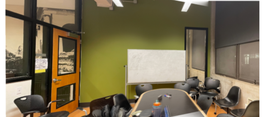
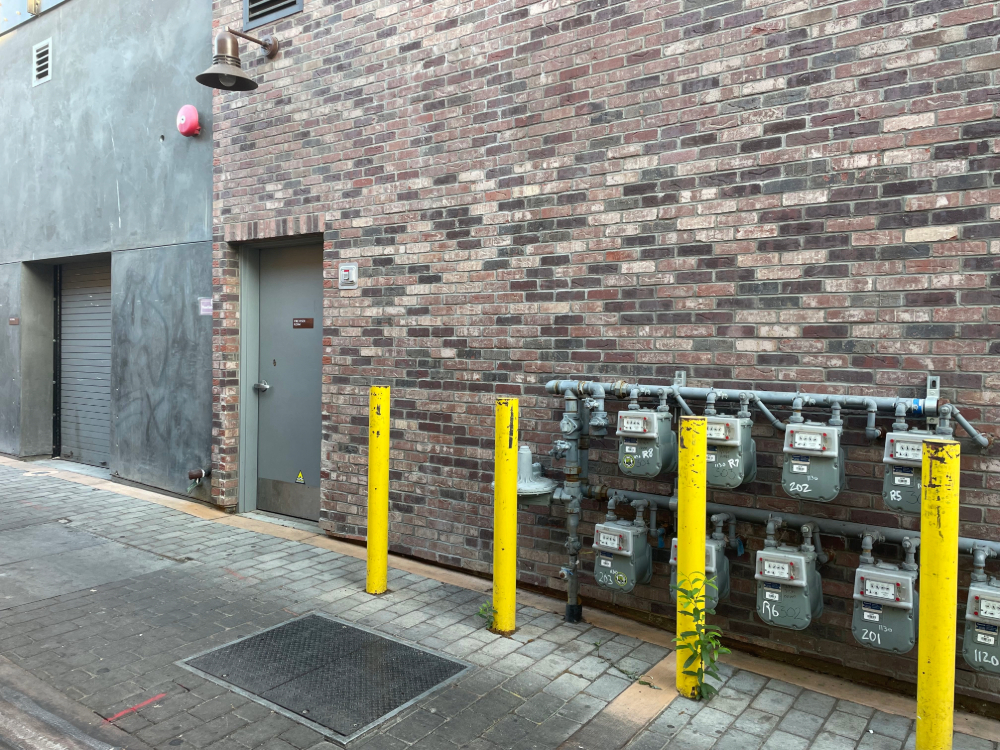
More base images:
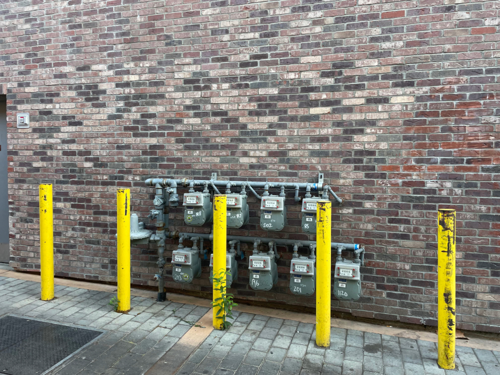
The final result!
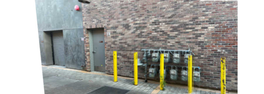
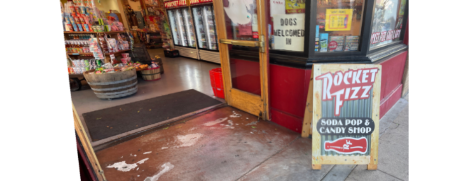
One last example with this storefront in downtown SLO.
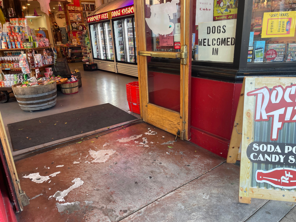
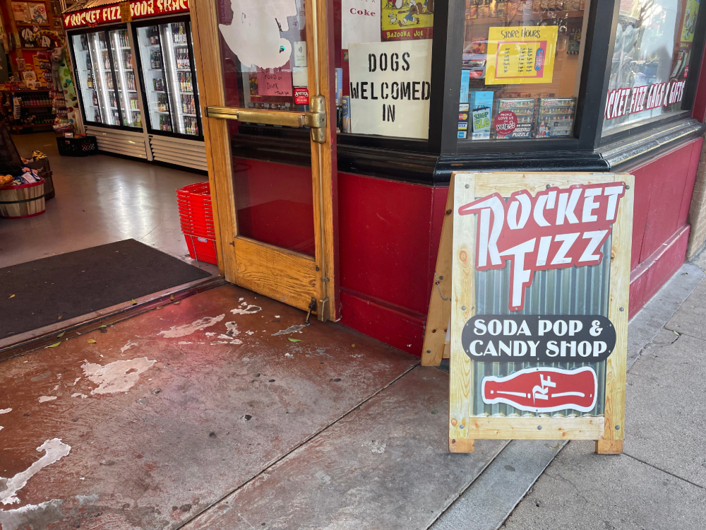
The final result!
The coolest thing I learned from this project is how easily the human visual perspective can be mimicked with a simple homography matrix! The features extraction was also interesting because of how it mimicks how humans pick out important points in images, and then how we use those points (although many, many more of them than in this project) to quickly merge one frame of our vision to the next.